At Unlearn, we develop various machine learning technologies for creating digital twins of individual patients. Specifically, a digital twin of a patient provides a comprehensive, probabilistic forecast of that patient’s future health. We refer to the machine learning models trained to generate digital twins of patients as digital twin generators. This post will provide a description of some of the machine learning methods used in the most recent versions of our digital twin generators. Please note that this post is somewhat technical and assumes some familiarity with common types of deep neural networks but doesn’t contain any mathematics—it’s medium technical. Also, Unlearn is an AI R&D organization and we’re constantly working on improvements to our model architectures so this is a representative example of some of our recent work in machine learning and not a definite description.

The Problem

While there are lots of potential applications of digital twins in medicine, we are primarily focused on applications within clinical trials. This narrows the problem space quite a bit. Our task is to use the data collected from a patient during their first visit in a clinical trial (the “baseline” data) to create a digital twin of the patient that forecasts how their clinical measurements would evolve over the course of the trial if they were given a placebo (or standard of care). Note that for this application we’re only forecasting how the patient’s clinical measurements would evolve on placebo, not how the patient might respond to a new experimental treatment. Therefore, we can train a digital twin generator for this task using longitudinal data collected from historical data of patients in the control groups of previous clinical trials or from disease registries.

To be a bit more concrete, let me give you an example. The dataset we used to build our digital twin generator for patients with Alzheimer’s disease incorporates data from over 30,000 patients aggregated from the control groups of dozens of clinical trials and some observational studies. Each patient in the dataset was observed in 3 to 6 month intervals for varying lengths of time up to 2 or 3 years. Taking into account both the number of patients and timepoints, the dataset has over 160,000 observations. Note we filter out some of these observations during model training due to data quality concerns, so the numbers in our spec sheets are a bit different.

One observation isn’t a single variable, however, rather it is a vector of 188 different clinical measurements. Many of these measurements are observed only infrequently, so we focused on a subset of 61 variables that have clinical importance and were measured frequently enough. Of these 61 variables, we consider 12 of them to be context variables that are only measured at baseline (e.g., sex, medical history, some biomarkers) and the remaining 49 variables (e.g., Alzheimer’s disease assessment scale components) are treated as longitudinal variables that change over time. Thus, our task is to train a model that takes the 12 context variables and 49 longitudinal variables at baseline as input and forecasts how the 49 longitudinal variables may change over time.

For a high dimensional timeseries like this, there are many metrics that we could use to determine if our model is doing a good job. Of course, we want to forecast the mean of each variable as a function of time. But we also want to forecast the standard deviation of each variable as a function of time in order to account for uncertainty, the correlations between all of the variables so that we can forecast linear combinations like composite scores, and time-lagged correlations so that we are accurately modeling the dynamics. That is, we want to train a probabilistic model that can generate realistic clinical trajectories. Then, we can calculate any summary statistics we are interested in by averaging over many sampled clinical trajectories for each patient.

Autoregressive Generative Models for Clinical Timeseries

To introduce generative models, it may be helpful to start with a simple analogy. In machine learning, we often say that there are two types of models: discriminative models and generative models. For example, a discriminative model could be trained to recognize if an image contains a picture of a cat, whereas a generative model could be trained to draw a picture of a cat. As another example, a discriminative model could be trained to recognize if a patient with Alzheimer’s disease is likely to progress relatively quickly or slowly, whereas a generative model could be trained to sample trajectories that represent possible future outcomes for that patient.

Generative models for sequential data are often autoregressive. For example, many language models are trained to predict the next word in a sequence given all of the words that came before it. Such a model can generate long sequences of words from an initial prompt by sampling the next word, adding it to the input, and repeating the process. While our models for clinical timeseries are different from those used in language models, they are also autoregressive generative models. The process of sampling from an autoregressive generative model is illustrated in the schematic below.

The High Level

At a very high level, one of our digital twin generators can be represented by the following architecture schematic.

This first schematic is highly simplified, but if you keep reading on I’ll reveal more of the components later on in the post.

The inputs to the model include all of the time-independent context variables, all of the longitudinal variables starting from baseline up until the current time, the times of all of the previous observations, and the future time that we want to forecast. The architecture that we’re currently using only relies on the observations at baseline and at the most recent timepoint; that is, it disgards information from intermediate timepoints. Dashed lines in the figure are used to represent the possibility that some variables may be missing at each timepoint.

The “black box predictor” in the figure uses the inputs to predict three things: the expected value of the longitudinal variables at the desired future time, the standard deviation of the longitudinal variables at the desired future time, and some statistics about the time to specific events (e.g., mean time to death). I’m being a bit loose with terminology here because this isn’t exactly how to interpret the outputs of the black box predictor, but it’s close enough for this post.

Although the black box predictor has many outputs, it’s not actually a generative model. We need a way to generate samples from a multivariate distribution with the predicted mean and standard deviation that also captures the correlations between the variables, and allows for variables that could be continuous or discrete. Thus, the outputs of the black box predictor become the parameters of a Neural Boltzmann Machine (NBM). Explaining how an NBM works is too much for this post, so if you’re interested check out our preprint on arxiv. For the time being, it’s sufficient to think of it as a type of neural network that takes a deterministic model like our black box predictor and turns it into a generative model for a probability distribution.

Inside the Black Box

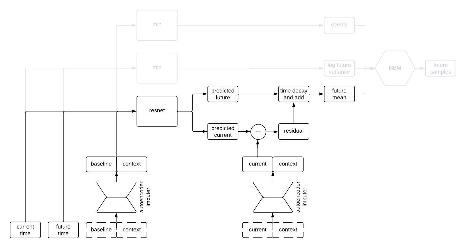
Alright, let’s peer inside the black box predictor. Here’s the full schematic, with the part I called a “black box predictor” previously now shown in red.

This is kind of a lot to take in, but I wanted to show the whole thing first. Now, let’s go through it piece by piece. The first component to tackle is the autoencoder imputer, highlighted below.

One common characteristic of healthcare data of all types is missingness. There are a variety of reasons for this, some of which are essentially insurmountable. As a result, it’s quite common that some of the inputs to the model won’t have been measured for a given patient; nevertheless, we still need to forecast their clinical trajectory.

An autoencoder is (typically) a type of neural network that learns to compress an input vector into a lower dimensional embedding and then to decompress the embedding in order to reconstruct the input. In order to faithfull compress and decompress the input, the autoencoder needs to learn the relationships between the various input variables. We use an autoencoder to impute missing data by replacing any missing variables with their reconstructed values. By adding the reconstruction loss of the autoencoder to the negative log likelihood of the NBM, we can train the network to impute missing data in a way that improves forecasting performance.  

The most normal looking part of the architecture is the point predictor, illustrated below.

The point predictor takes the data from a patient at baseline, the contextual information, and two times we call the current time and the future time (where the current time comes before the future time), and it outputs predictions for the longitudinal variables at the current and future times. The prediction comes from a residual network, which essentially means a neural network that is predicting the change from baseline. This looks like a normal prediction model, except we query it twice to get predictions for two different timepoints.

Why do we query the prediction model twice, you ask? We’re going to use the two predictions, at two different timepoints, in order to incorporate autocorrelations in the generated clinical trajectories. Suppose we make two predictions for a patient, one 90 days into a study and the other 91 days into the study. Then, we observe that our prediction for some variable—say, the patient’s weight—was too low at day 90. Maybe we predicted them to weigh 160 pounds, but they actually weighed 175 pounds. Is our prediction for their weight on day 91 likely to be too high or too low? Well, if it was too low on day 90 then it’s probably still too low on day 91. That is, the errors (or residuals) for the predictions at two timepoints are likely to be similar if those times are close together. That’s an autocorrelation.

To incorporate autocorrelations into our generated trajectories, we take the predicted values for the longitudinal variables at the current time and subtract their observed/imputed values to compute a residual, then we multiply the residual by a function that decays with the difference between the current and future times and add it to our prediction for the future time. This gives us a prediction for the expected value of the longitudinal variables at the future time given the observations at the previous times. This is illustrated in the schematic below.

I like to think of this model as having a type of hard-coded attention mechanism. Regardless of how long the sequence is, the prediction network always uses the information from the baseline and current time and discards the information from intermediate times. This makes sense for our clinical trial applications because one usually only gets information about a patient from a single time point (i.e, at baseline) so we want to remember that information indefinitely. A different, more typical, attention mechanism could make sense if, for example, we were inputting long sequences of each patient’s medical history.

The next part of the network I’d like to highlight in the figure above is the part that predicts the standard deviation of each longitudinal variable at the future time. This network is a multilayer perceptron (a.k.a., a regular ol’ neural network, MLP) that takes the output of the autoencoder imputer applied to the baseline and context as well as the current and future times, and outputs the logarithm of the variance at the future time.

Why does it take both the current and future times? Since we are sampling autoregressively, if the current and future times are close together then we expect the standard deviation of the conditional distribution to be small, whereas we expect the standard deviation to be large if the two times are far apart. Therefore, we use the MLP to predict the variance at the future time from the baseline and context variables, and then shrink it towards zero by an amount that depends on the difference between the current and future times.

The final piece of the prediction module is a time-to-event model that we include for indications in which there are specific clinical events to predict. We use an accelerated failure time model computed using an MLP from the imputed baseline and context vectors.

So, that’s all of the basic components. The final architecture looks something like this:

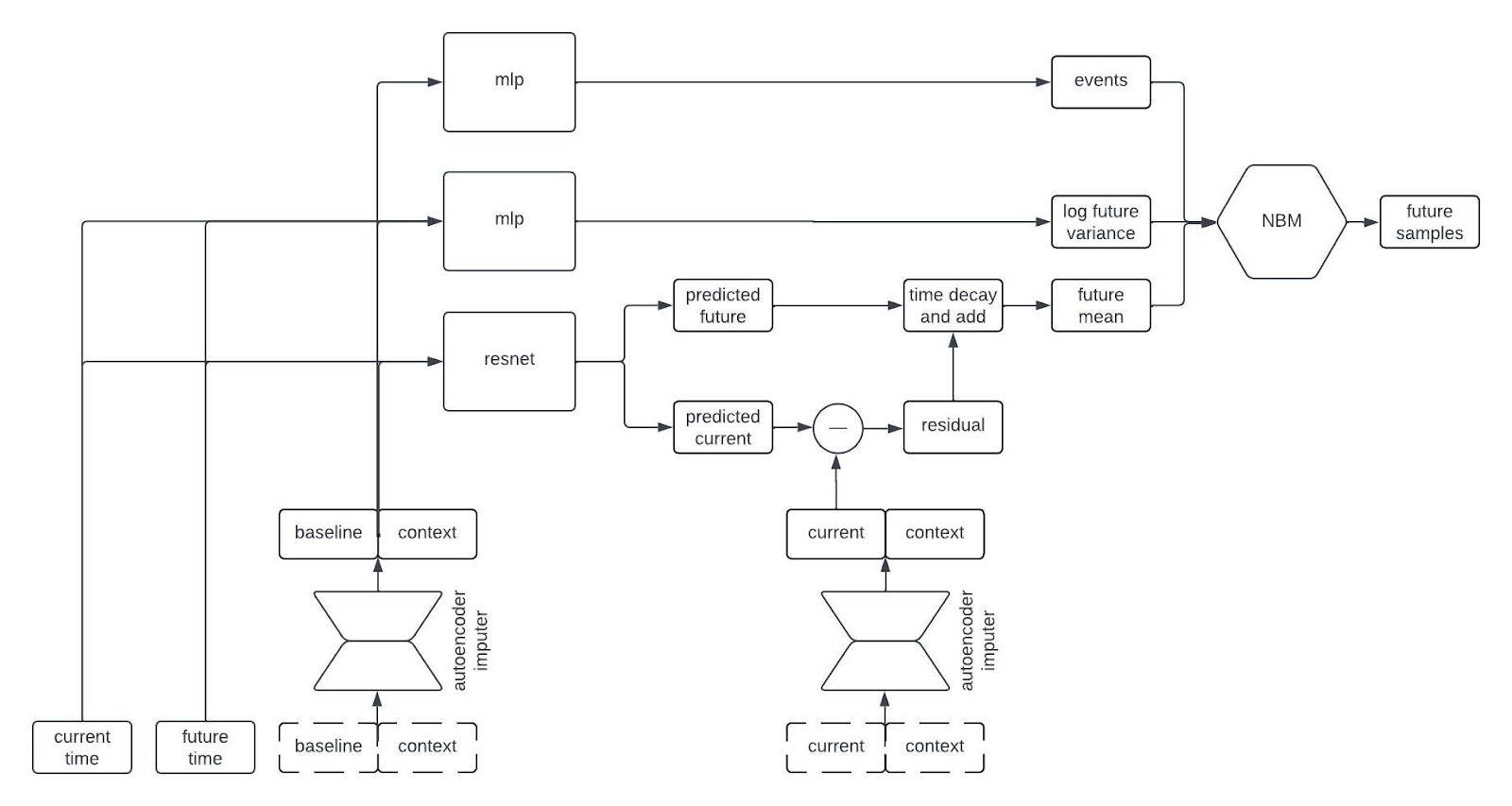
We train these models by minimizing a composite loss function that combines the reconstruction error of the autoencoder, the negative log likelihood of the NBM, and the negative log likelihood of the time-to-event model. Note that there is no explicit loss on the network module that predicts the future mean or the network module that predicts the log of the future variance as both of those are fully accounted for in the loss function of the NBM. As in most applications of deep neural networks, we also apply various regularization techniques to the architecture during training.

Why this architecture?

The digital twin generator architecture I’ve described produces continuous time, probabilistic forecasts of multivariate clinical timeseries from a single observation at baseline and some contextual information. In addition to having new capabilities, using fewer computing resources, and generally achieving higher performance than our previous architectures, our new NBM based architectures have some other advantages. In particular, the architecture is simultaneously highly modular while also being end-to-end differentiable. As a result, it’s quite easy to swap out one module for another, which has sped up our iteration time on R&D dramatically. I imagine that this blog post will be outdated 6 months from now, and that’s the way it should be.